Diffusion equation in TCLB solver
Contents
Diffusion equation in TCLB solver
In this workshop we will cover basic conceptions related to TCLB solver. We will not dive into detail of TCLB compilation or model development - it is out of scope of this tutorial and is covered in other materials.
The d2q9_reaction_diffusion_system_XXXX models
This TCLB model is a collection of Reaction-Diffusion Partial/Ordinary differential equations systems. Basically, the model is build to solve systems in form:
Where \(DRE_1(x,t)\) is spatially variable field, solution of first Diffusion-Reaction equation, and \(ODE_1(x,t)\) is solution of Ordinary Differential Equation at point \(x\). Both equations are solved using second order, implicit midpoint scheme. Spatial discretisation of DRE is performed using LBM method - details could be found in [X]. The right hend side vector is equall $\( \mathbb{RHS} = \left[ DRE_i(x,t), ODE_i(x,t) \right] \)$
Most of the models have meaningfull names for \(\mathbf{DRE_i}\) variables and params, provided below.
At point of writing, supported model are:
d2q9_reaction_diffusion_system_SimpleDiffusion
or
d2q9_reaction_diffusion_system_AllenCahn
or
d2q9_reaction_diffusion_system_SIR_SimpleLaplace
This simple spatial extension of SIR model, by addition of diffusivity $\(\nabla \left( S,I,R \right)\)$ to every term
or
for \(N=1\)
d2q9_reaction_diffusion_system_SIR_ModifiedPeng
or the WSIR model, aleready referenced in this workshop
or
Keep in mind that for consistency, it’s recomended to set $\( \mathbf{Diffusivity\_W} = \mathbf{Beta_w} * \frac{r^2}{8} \)$
Additionally, list of models could be extracted via:
! tclbmake d2q9_reaction_diffusion_system/list
TCLB_PATH:  /home/mdzik/_TCLB/TCLB
                                                 AllenCahn SIR_ModifiedPeng
d2q9_reaction_diffusion_system_AllenCahn                 X                -
d2q9_reaction_diffusion_system_SIR_ModifiedPeng          -                X
d2q9_reaction_diffusion_system_SIR_SimpleLaplace         -                -
d2q9_reaction_diffusion_system_SimpleDiffusion           -                -
                                                 SIR_SimpleLaplace
d2q9_reaction_diffusion_system_AllenCahn                         -
d2q9_reaction_diffusion_system_SIR_ModifiedPeng                  -
d2q9_reaction_diffusion_system_SIR_SimpleLaplace                 X
d2q9_reaction_diffusion_system_SimpleDiffusion                   -
                                                 SimpleDiffusion
d2q9_reaction_diffusion_system_AllenCahn                       -
d2q9_reaction_diffusion_system_SIR_ModifiedPeng                -
d2q9_reaction_diffusion_system_SIR_SimpleLaplace               -
d2q9_reaction_diffusion_system_SimpleDiffusion                 X
What is included in this environment
To run TCLB model us ipython shell binding:
! tclb ModelName ConfigurationFile.xml
This will effectivelu run (in the curren working directory)
$TCLB_PATH/CLB/ModelName/main ConfigurationFile.xml
in your Jupyter/Binder. We will use
! tclb ModelName ConfigurationFile.xml > /dev/null && echo "DONE!"
to supress output in most cases.
TCLB solver
As you might noticed TCLB is a set of models (like d2q9). TCLB uses XML as source of configuration plus limited numebr of command line options which will be covered latter. There is a python library that helps you build XML on-the-fly if You like.
import h5py
import numpy as np
import matplotlib.pyplot as plt
from display_xml import XML
Basic configuration file
Let’s solve diffusion equation, on 100x100 domain with diffusivity \(\nu=1/6\)
<CLBConfig version="2.0" output="output/SimpleDiffusion/"> <!-- The root xml element -->
  <Geometry nx="100" ny="100"> <!-- Mesh size, by default nz=1. MPI divisions are along X -->
    <None name="city"> <!--Named zone or BC, part of the mesh that could be referenced in Model section  -->
      <Box dx="35" nx="30"/> <!-- Markers/geometrical descriptions of the parent zone -->
    </None>
  </Geometry>
  <Model> <!-- Here we set the model parameters, like viscosity -->
    <Param name="Diffusivity_DRE_1" value="0.1666"/> <!-- or Diffusivity for Diffusive-Reactive-Equation #1  -->
    <Param name="Init_DRE_1" value="-0.5"/> <!-- Initial value for Diffusive-Reactive-Equation #1  -->
    <Param name="Init_DRE_1" value="0.5" zone="city"/> <!-- Initial value for Diffusive-Reactive-Equation #1  in Zone City -->
  </Model>
  <HDF5/> <!-- Save at t=0  -->
  <Solve Iterations="200"> <!-- Iterate 100 iterations -->
    <HDF5 Iterations="10"/> <!-- Save HDF5 every 10, HDF5 could be replaced by VTK -->
  </Solve>
</CLBConfig>
and let’s run it:
! tclb d2q9_reaction_diffusion_system_SimpleDiffusion SimpleDiffusion.xml
MPMD: TCLB: local:0/1 work:0/1 ---  connected to:
[  ] -------------------------------------------------------------------------
[  ] -  CLB version:       v6.5.0-71-g352b9281                               -
[  ] -        Model: d2q9_reaction_diffusion_system_SimpleDiffusion
[  ]              -
[  ] -------------------------------------------------------------------------
[  ] Setting output path to: SimpleDiffusion
[  ] Discarding 1 comments
[ 0] Running on CPU
[ 0] WARNING: No "Units" element in config file
[  ] Mesh size in config file: 100x100x1
[  ] Global lattice size: 100x100x1
[  ] Max region size: 10000. Mesh size 10000. Overhead:  0%
[  ] Local lattice size: 100x100x1
Hello allocator!
[  ]   Threads  |      Action
[  ]     1x1    | Primal , NoGlobals , InitFromExternal
[  ]     1x1    | Tangent , NoGlobals , InitFromExternal
[  ]     1x1    | Optimize , NoGlobals , InitFromExternal
[  ]     1x1    | SteadyAdjoint , NoGlobals , InitFromExternal
[  ]     1x1    | Primal , IntegrateGlobals , InitFromExternal
[  ]     1x1    | Tangent , IntegrateGlobals , InitFromExternal
[  ]     1x1    | Optimize , IntegrateGlobals , InitFromExternal
[  ]     1x1    | SteadyAdjoint , IntegrateGlobals , InitFromExternal
[  ]     1x1    | Primal , OnlyObjective , InitFromExternal
[  ]     1x1    | Tangent , OnlyObjective , InitFromExternal
[  ]     1x1    | Optimize , OnlyObjective , InitFromExternal
[  ]     1x1    | SteadyAdjoint , OnlyObjective , InitFromExternal
[  ]     1x1    | Primal , NoGlobals , BaseIteration
[  ]     1x1    | Tangent , NoGlobals , BaseIteration
[  ]     1x1    | Optimize , NoGlobals , BaseIteration
[  ]     1x1    | SteadyAdjoint , NoGlobals , BaseIteration
[  ]     1x1    | Primal , IntegrateGlobals , BaseIteration
[  ]     1x1    | Tangent , IntegrateGlobals , BaseIteration
[  ]     1x1    | Optimize , IntegrateGlobals , BaseIteration
[  ]     1x1    | SteadyAdjoint , IntegrateGlobals , BaseIteration
[  ]     1x1    | Primal , OnlyObjective , BaseIteration
[  ]     1x1    | Tangent , OnlyObjective , BaseIteration
[  ]     1x1    | Optimize , OnlyObjective , BaseIteration
[  ]     1x1    | SteadyAdjoint , OnlyObjective , BaseIteration
[  ]     1x1    | Primal , NoGlobals , BaseInit
[  ]     1x1    | Tangent , NoGlobals , BaseInit
[  ]     1x1    | Optimize , NoGlobals , BaseInit
[  ]     1x1    | SteadyAdjoint , NoGlobals , BaseInit
[  ]     1x1    | Primal , IntegrateGlobals , BaseInit
[  ]     1x1    | Tangent , IntegrateGlobals , BaseInit
[  ]     1x1    | Optimize , IntegrateGlobals , BaseInit
[  ]     1x1    | SteadyAdjoint , IntegrateGlobals , BaseInit
[  ]     1x1    | Primal , OnlyObjective , BaseInit
[  ]     1x1    | Tangent , OnlyObjective , BaseInit
[  ]     1x1    | Optimize , OnlyObjective , BaseInit
[  ]     1x1    | SteadyAdjoint , OnlyObjective , BaseInit
[  ] [0] Cumulative allocation of 1619520 b (1.6 MB)
[  ] Creating geom size:10000
[  ] Setting output path to: SimpleDiffusion
[  ] Setting output path to: output/SimpleDiffusion/SimpleDiffusion
[  ] loading geometry ...
[  ] Setting number of zones to 2
[  ] Setting Diffusivity_PHI to 0.1666 (0.166600)
[  ] [0] Settings [Diffusivity for _PHI] to 0.166600
[  ] Setting Init_PHI in zone  (-1) to -0.5 (-0.500000)
[  ] Setting Init_PHI in zone city (1) to 0.5 (0.500000)
[  ] Initializing Lattice ...
[  ] Callback HDF5 with no Iterations attribute==] 2373h  2m
[  ] Negotiated HDF5 chunks: 1x100x100[x3]
[  ]        0 it writing hdf5
[  ] Setting action Solve at 200.000000 iterations
[  ] Setting callback HDF5 at 10.000000 iterations
[  ] Negotiated HDF5 chunks: 1x100x100[x3]
[  ] Adding HDF5 to the solver hands
[  ]     53.0 MLBUps      8.58 GB/s [====================]2m
[  ]       10 it writing hdf5
[  ]     53.9 MLBUps      8.74 GB/s [====================]
[  ]       20 it writing hdf5
[  ]     17.8 MLBUps      2.89 GB/s [====================]
[  ]       30 it writing hdf5
[  ]     17.7 MLBUps      2.86 GB/s [====================]
[  ]       40 it writing hdf5
[  ]     17.8 MLBUps      2.88 GB/s [====================]
[  ]       50 it writing hdf5
[  ]     17.5 MLBUps      2.84 GB/s [====================]
[  ]       60 it writing hdf5
[  ]     17.4 MLBUps      2.83 GB/s [====================]
[  ]       70 it writing hdf5
[  ]     16.2 MLBUps      2.62 GB/s [====================]
[  ]       80 it writing hdf5
[  ]     17.5 MLBUps      2.84 GB/s [====================]
[  ]       90 it writing hdf5
[  ]      7.4 MLBUps      1.20 GB/s [====================]
[  ]      100 it writing hdf5
[  ]     16.8 MLBUps      2.72 GB/s [====================]
[  ]      110 it writing hdf5
[  ]     18.0 MLBUps      2.92 GB/s [====================]
[  ]      120 it writing hdf5
[  ]     18.1 MLBUps      2.93 GB/s [====================]
[  ]      130 it writing hdf5
[  ]     18.2 MLBUps      2.95 GB/s [====================]
[  ]      140 it writing hdf5
[  ]     18.8 MLBUps      3.05 GB/s [====================]
[  ]      150 it writing hdf5
[  ]     18.8 MLBUps      3.05 GB/s [====================]
[  ]      160 it writing hdf5
[  ]      8.3 MLBUps      1.35 GB/s [====================]
[  ]      170 it writing hdf5
[  ]     18.5 MLBUps      2.99 GB/s [====================]
[  ]      180 it writing hdf5
[  ]     17.8 MLBUps      2.88 GB/s [====================]
[  ]      190 it writing hdf5
[  ]     18.4 MLBUps      2.98 GB/s [====================]
[  ]      200 it writing hdf5
[  ] Total duration: 1.161041 s = 0.019351 min = 0.000323 h
TimeSteps = list()
for i in range(0,200,10):
f = h5py.File('./output/SimpleDiffusion/SimpleDiffusion_HDF5_%08d.h5'%i)
TimeSteps.append(f['PHI'][0,:,:])
TimeSteps = np.array(TimeSteps)
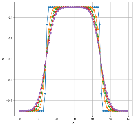
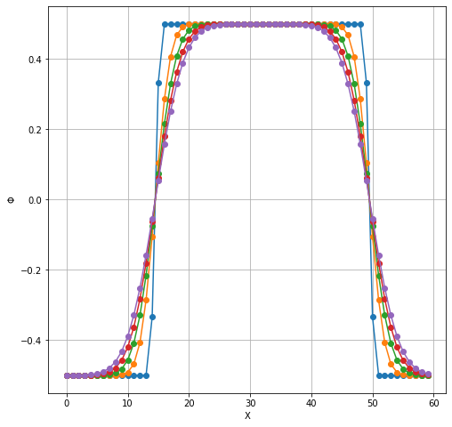
plt.figure(figsize=(8,8))
plt.plot(TimeSteps[:5,25,20:80].T, 'o-');
plt.grid(which='both');
plt.xlabel('X');
plt.ylabel(r'$\Phi$');
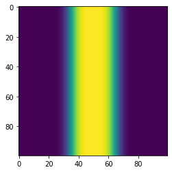
We could also extract 1D image
plt.imshow(TimeSteps[5])
<matplotlib.image.AxesImage at 0x7fde646a9f40>
Using TCLBConfig writer class
Now, we are gona generate same XML file using XML library. A nice think is that we could use it to do some parametric studies. It also does limited “syntax” check.
import CLB.CLBXMLWriter as CLBXML
CLBc = CLBXML.CLBConfigWriter( )

CLBc.addGeomParam('nx', 100)
CLBc.addGeomParam('ny', 100)

CLBc.addNone(name="city")
CLBc.addBox(dx=35, nx=35)

params = {
        "Diffusivity_PHI":0.1666,
        "Init_PHI":-0.5
}

CLBc.addModelParams(params)

params = {
        "Init_PHI":0.5
}

CLBc.addHDF5()
CLBc.addModelParams(params, zone='city')
solve = CLBc.addSolve(iterations=200)
CLBc.addHDF5(Iterations=10, parent=solve)

CLBc.write('SimpleDiffusionByCLBXMLWriter.xml')
Apart from float representation, the resulting file is identical
f = open('SimpleDiffusionByCLBXMLWriter.xml', 'r')
XML(''.join(f.readlines()))
<CLBConfig version="2.0" output="output/">
  <!--Created using CLBConfigWriter-->
  <Geometry predef="none" model="MRT" nx="100.0000000000000000" ny="100.0000000000000000">
    <None name="city">
      <Box dx="35" nx="35"/>
    </None>
  </Geometry>
  <Model>
    <Param name="Diffusivity_PHI" value="0.1666000000000000"/>
    <Param name="Init_PHI" value="-0.5000000000000000"/>
    <Param name="Init_PHI" value="0.5000000000000000" zone="city"/>
  </Model>
  <HDF5/>
  <Solve Iterations="200">
    <HDF5 Iterations="10"/>
  </Solve>
</CLBConfig>
! tclb d2q9_reaction_diffusion_system_SimpleDiffusion SimpleDiffusionByCLBXMLWriter.xml > /dev/null && echo "DONE!"
Hello allocator!
DONE!
TimeSteps2 = list()

for i in range(0,200,10):
    f = h5py.File('./output/SimpleDiffusionByCLBXMLWriter_HDF5_%08d.h5'%i)
    TimeSteps2.append(f['PHI'][0,:,:])

TimeSteps2 = np.array(TimeSteps2)

plt.figure(figsize=(8,8))
plt.plot(TimeSteps2[:5,25,20:80].T, 'o-');
plt.grid(which='both');
plt.xlabel('X');
plt.ylabel(r'$\Phi$');
RInside: periodic IC and comparison with Finite Difference
Let’s create initial condition, we will start in python
R inside block is build as
CLBc.addRunR(eval=\
"""
some <- r_code
""")
which will result in XML as:
<RunR>
<![CDATA[
   some <- r_code
]]>
</RunR>
Notice, that < in some cases got converted into <. This is XML character escaping. Keep the CDATA element and all be OK :)
Outmost usable part of R-TCLB integration are accessors to internal Fields:
r Solver.Fields.FIELDNAME[] = SAMESHAPEVARIABLE;
and Actions/Stages:
Solver.Actions.InitFromExternalAction();
You could also call standard R functions inside (Full R should be avalible - it’s embeded interpreter, see RInside upstream documentation for details/limitations if you need):
init = read.table("initial.csv", header = FALSE, sep = "", dec = ".");
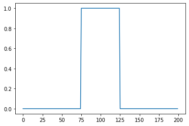
Let’s create initial “data file”
u_ic = np.zeros(200)
u_ic[75:-75] = 1
plt.plot(u_ic)
np.savetxt("initial.csv", u_ic, delimiter=",")
Now the XML configuration
CLBc = CLBXML.CLBConfigWriter( )

CLBc.addGeomParam('nx', 200)
CLBc.addGeomParam('ny', 100)


CLBc.addRunR(eval=\
"""
    init = read.table("initial.csv", header = FALSE, sep = "", dec = ".");
    Solver$Fields$Init_PHI_External[] = init[,1];
    Solver$Actions$InitFromExternalAction();
""")


params = {
        "Diffusivity_PHI":0.1666,
        "Init_PHI":-0.5
}

CLBc.addModelParams(params)


CLBc.addHDF5()
solve = CLBc.addSolve(iterations=200)
CLBc.addHDF5(Iterations=10, parent=solve)

CLBc.write('SimpleDiffusionWithRinside.xml')

f = open('SimpleDiffusionWithRinside.xml', 'r')
XML(''.join(f.readlines()))
<CLBConfig version="2.0" output="output/">
  <!--Created using CLBConfigWriter-->
  <Geometry predef="none" model="MRT" nx="200.0000000000000000" ny="100.0000000000000000"/>
  <Model>
    <Param name="Diffusivity_PHI" value="0.1666000000000000"/>
    <Param name="Init_PHI" value="-0.5000000000000000"/>
  </Model>
  <RunR>
    init = read.table("initial.csv", header = FALSE, sep = "", dec = ".");
    Solver$Fields$Init_PHI_External[] = init[,1];
    Solver$Actions$InitFromExternalAction();
</RunR>
  <HDF5/>
  <Solve Iterations="200">
    <HDF5 Iterations="10"/>
  </Solve>
</CLBConfig>
! tclb d2q9_reaction_diffusion_system_SimpleDiffusion SimpleDiffusionWithRinside.xml > /dev/null && echo 'DONE!'
Hello allocator!
DONE!
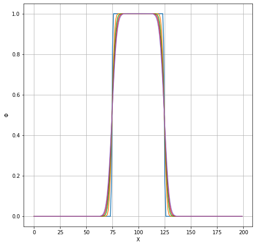
Solution obtained from TCLB
TimeSteps2 = list()

for i in range(0,200,10):
    f = h5py.File('./output/SimpleDiffusionWithRinside_HDF5_%08d.h5'%i)
    TimeSteps2.append(f['PHI'][0,:,:])

TimeSteps2 = np.array(TimeSteps2)

plt.figure(figsize=(8,8))
plt.plot(TimeSteps2[:5,25,:].T, '-');
plt.grid(which='both');
plt.xlabel('X');
plt.ylabel(r'$\Phi$');
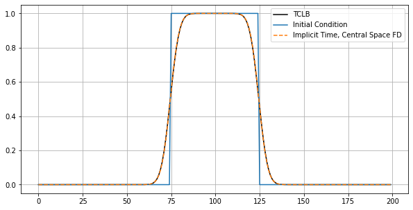
Comparison with Backward Time - Central Space FD
def btcs(u_IC, nu, nx, nt, dt, dx):

    un_icfd = u_IC.copy()
    A = np.zeros((nx, nx))


    Beta_FD = dt * nu / (dx**2)
    # nt += 100
    last_index_in_matrix = nx -1
    # the BC  - use one sided FD
    A[0, 0] = 1-Beta_FD     # forward FD
    A[0, 1] = 2*Beta_FD     # forward FD
    A[0, 2] = -Beta_FD      # forward FD
    A[last_index_in_matrix, last_index_in_matrix-2] = -Beta_FD   # backward FD
    A[last_index_in_matrix, last_index_in_matrix-1] = 2*Beta_FD  # backward FD
    A[last_index_in_matrix, last_index_in_matrix] =  1-Beta_FD   # backward FD
    for i in range(1, last_index_in_matrix):
        A[i, i-1] = -Beta_FD        # left of the diagonal
        A[i, i] = 1 + 2*Beta_FD     # the diagonal
        A[i, i+1] = -Beta_FD         # right of the diagonal

    A_inv = np.linalg.inv(A)
    solution = list()
    solution.append(u_ic)
    for n in range(nt):  #loop for values of n from 0 to nt, so it will run nt times
        un_icfd = A_inv@un_icfd
        solution.append(un_icfd)

    return np.array(solution)


solution = btcs(u_ic, 0.1666, u_ic.shape[0], 200, 1, 1)
plt.figure(figsize=(10,5))
plt.plot(TimeSteps2[5,25,:].T, 'k-', label='TCLB');
plt.plot(solution[0,:], label='Initial Condition')
plt.plot(solution[50,:], '--', label='Implicit Time, Central Space FD')
plt.legend()
plt.grid(which='both')
RInside: read an image as initial condition
Firstly - we need to install locally aditional R package - jpeg, to enable us interaction with JPEG files. We could install it locally, bu keep it mind, that if you are using it at BinderHub, this is temparary
! mkdir -p r_packages
! echo 'install.packages("jpeg", repos="http://cran.r-project.org", lib="r_packages")' | /usr/bin/R --slave
trying URL 'http://cran.r-project.org/src/contrib/jpeg_0.1-9.tar.gz'
Content type 'application/x-gzip' length 18596 bytes (18 KB)
==================================================
downloaded 18 KB

* installing *source* package 'jpeg' ...
** package 'jpeg' successfully unpacked and MD5 sums checked
** using staged installation
** libs
gcc -std=gnu99 -I"/usr/share/R/include" -DNDEBUG     -fpic  -g -O2 -fdebug-prefix-map=/build/r-base-jbaK_j/r-base-3.6.3=. -fstack-protector-strong -Wformat -Werror=format-security -Wdate-time -D_FORTIFY_SOURCE=2 -g  -c read.c -o read.o
gcc -std=gnu99 -I"/usr/share/R/include" -DNDEBUG     -fpic  -g -O2 -fdebug-prefix-map=/build/r-base-jbaK_j/r-base-3.6.3=. -fstack-protector-strong -Wformat -Werror=format-security -Wdate-time -D_FORTIFY_SOURCE=2 -g  -c reg.c -o reg.o
gcc -std=gnu99 -I"/usr/share/R/include" -DNDEBUG     -fpic  -g -O2 -fdebug-prefix-map=/build/r-base-jbaK_j/r-base-3.6.3=. -fstack-protector-strong -Wformat -Werror=format-security -Wdate-time -D_FORTIFY_SOURCE=2 -g  -c write.c -o write.o
gcc -std=gnu99 -shared -L/usr/lib/R/lib -Wl,-Bsymbolic-functions -Wl,-z,relro -o jpeg.so read.o reg.o write.o -ljpeg -L/usr/lib/R/lib -lR
installing to /home/mdzik/_TCLB/TCLB_binder/IDUB/workshops/40_draft_IntroTCLB/r_packages/00LOCK-jpeg/00new/jpeg/libs
** R
** inst
** byte-compile and prepare package for lazy loading
** help
*** installing help indices
** building package indices
** testing if installed package can be loaded from temporary location
** checking absolute paths in shared objects and dynamic libraries
** testing if installed package can be loaded from final location
** testing if installed package keeps a record of temporary installation path
* DONE (jpeg)

The downloaded source packages are in
	'/tmp/Rtmpy76tOo/downloaded_packages'
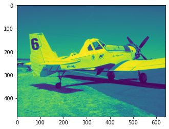
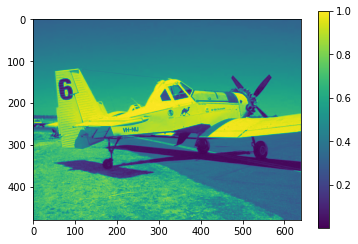
Let’s check if it work - we use an image of a M-18A Dromader airplane as initial condition ;)
CLBc = CLBXML.CLBConfigWriter( )

CLBc.addGeomParam('nx', 640)
CLBc.addGeomParam('ny', 480)


CLBc.addRunR(eval=\
"""
    library('jpeg', lib="r_packages")

    myurl <- "https://upload.wikimedia.org/wikipedia/commons/thumb/a/a5/M-18A_Dromader_CALM.jpg/640px-M-18A_Dromader_CALM.jpg"
    z <- tempfile()
    download.file(myurl,z,mode="wb", quiet=TRUE);
    pic <- readJPEG(z);
    file.remove(z) # cleanup

    Solver$Fields$Init_PHI_External[] = t(pic[,,1]);
    Solver$Actions$InitFromExternalAction();
""")


params = {
        "Diffusivity_PHI":0.1666,
        "Init_PHI":-0.5
}

CLBc.addModelParams(params)

CLBc.addHDF5()
CLBc.write('SimpleDiffusionOfDromader.xml')


! tclb d2q9_reaction_diffusion_system_SimpleDiffusion SimpleDiffusionOfDromader.xml > /dev/null && echo "DONE"

i = 0
f = h5py.File('./output/SimpleDiffusionOfDromader_HDF5_%08d.h5'%i)
plt.imshow(f['PHI'][0,:,:])
plt.colorbar()
Hello allocator!
DONE
<matplotlib.colorbar.Colorbar at 0x7fde64a98460>
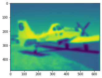
The CLBc object could be reused (something could be appended to it after save, parameters could bo overwritten)
XML for diffusion of the example image will look like that:
solve = CLBc.addSolve(iterations=200)
CLBc.addHDF5(Iterations=10, parent=solve)
CLBc.write('SimpleDiffusionOfDromader_withIterations.xml')
f = open('SimpleDiffusionOfDromader_withIterations.xml', 'r')
XML(''.join(f.readlines()))
<CLBConfig version="2.0" output="output/">
<!--Created using CLBConfigWriter-->
<Geometry predef="none" model="MRT" nx="640.0000000000000000" ny="480.0000000000000000"/>
<Model>
<Param name="Diffusivity_PHI" value="0.1666000000000000"/>
<Param name="Init_PHI" value="-0.5000000000000000"/>
</Model>
<RunR>
library('jpeg', lib="r_packages")
myurl <- "https://upload.wikimedia.org/wikipedia/commons/thumb/a/a5/M-18A_Dromader_CALM.jpg/640px-M-18A_Dromader_CALM.jpg"
z <- tempfile()
download.file(myurl,z,mode="wb", quiet=TRUE);
pic <- readJPEG(z);
file.remove(z) # cleanup
Solver$Fields$Init_PHI_External[] = t(pic[,,1]);
Solver$Actions$InitFromExternalAction();
</RunR>
<HDF5/>
<Solve Iterations="200">
<HDF5 Iterations="10"/>
</Solve>
</CLBConfig>
! tclb d2q9_reaction_diffusion_system_SimpleDiffusion SimpleDiffusionOfDromader_withIterations.xml > /dev/null && echo "DONE"
Hello allocator!
DONE
for i in range(0,200,50):
    plt.figure()
    f = h5py.File('./output/SimpleDiffusionOfDromader_withIterations_HDF5_%08d.h5'%i)
    plt.imshow(f['PHI'][0,:,:])