First shot: spatially variable SIR model with uniform IC¶

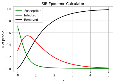
To evaluate, if model is working, let’s start with basic case: uniform initial distribution of SIR variables, with periodic BC. This should give solution for original SIR ODE, if \(\beta\) is sufficiently large.

Firstly, we prepare solution of ODE using SymPy’s solve_ivp toolbox. For details see previous workshops.

#Test case settings

I_init = 0.3
S_init = 1. - I_init
R_init = 0
Beta = 5
Gamma = 1
T = 5



###########################3
# FD SOLUTION #


def SIR_0D(t, z, beta, gamma, N):
    """
     # Susceptible → Infected → Removed
    :param t: time [days]
    :param z: Susceptible, Exposed, Infected, Removed
    :param beta: average number of contacts per day for each infected individual
    :param gamma: Between I and R, the transition rate is γ
    (simply the frequency of recoveries, that is, number of recovered or dead during one day
    divided by the total number of infected on that same day, supposing "day" is the time unit).
    If the duration of the infection is denoted D, then γ = 1/D.
    :return: derivatives [dS, dI, dR]
    """

    S, I, R = z
    dSdt = -beta*I*S/N
    dIdt = beta*I*S/N - I*gamma
    dRdt = I*gamma
    return [dSdt, dIdt, dRdt]



# INITIAL CONDItIONS
initial_susceptible = S_init # initial number of susceptible individuals in population.
initial_infections = I_init  # initial number of infected individuals in population.
initial_removed = R_init  # initial number of removed (recovered) individuals in population.
IC = np.array([initial_susceptible, initial_infections, initial_removed])

days_to_simulate = T
sol = solve_ivp(SIR_0D,
                [0, days_to_simulate],
                IC,
                method='RK45',
                args=[Beta, Gamma, 1],
                dense_output=True)

t_rk4 = np.linspace(0, days_to_simulate, 1000)
z = sol.sol(t_rk4)

S_rk4, I_rk4, R_rk4 = z

params = {'legend.fontsize': 'xx-large',
          'figure.figsize': (14, 8),
         'axes.labelsize': 'xx-large',
         'axes.titlesize':'xx-large',
         'xtick.labelsize':'xx-large',
         'ytick.labelsize':'xx-large'}
axes = plt.gca()
plt.plot(t_rk4, S_rk4,
         color="green", marker="", markevery=1, markersize=15, linestyle="-", linewidth=2,
         label='Susceptible')
plt.plot(t_rk4, I_rk4,
         color="red", marker="", markevery=1, markersize=15, linestyle="-", linewidth=2,
         label='Infected')
plt.plot(t_rk4, R_rk4,
         color="black", marker="", markevery=1, markersize=15, linestyle="-", linewidth=2,
         label='Removed')


plt.xlabel('t')
plt.ylabel('% of people')
plt.title('SIR Epidemic Calculator')
plt.legend()
plt.grid()

plt.show()

# plt.plot(t_rk4, S_rk4,
#          color="green", marker="", markevery=1, markersize=15, linestyle="-", linewidth=2,
#          label='S - RK45')
# plt.plot(t_rk4, I_rk4,
#          color="red", marker="", markevery=1, markersize=15, linestyle="-", linewidth=2,
#          label='I - RK45')
# plt.plot(t_rk4, R_rk4,
#          color="black", marker="", markevery=1, markersize=15, linestyle="-", linewidth=2,
#          label='R - RK45')
# plt.legend()

../../_images/15_d2q9_diffusion_SpatialSIR_model_3_0.png

We will use d2q9_reaction_diffusion_system_SIR_ModifiedPeng model (or the WSIR model), aleready referenced in this workshop

\[\begin{split} \frac{\partial}{\partial t} W = \beta_W \left[\frac{r^2}{8}W + (I-W) \right] \\ \frac{\partial}{\partial t} S = - \beta \frac{S}{N}W\\ \frac{\partial}{\partial t} I = \beta \frac{S}{N}W - \gamma I \\ \frac{\partial}{\partial t} R = \gamma I \end{split}\]

where

\[\begin{split} S = ODE_1 \\ I = ODE_2 \\ R = ODE_3 \\ C_1 = R_0 \\ C_2 = \beta\\ C_3 = dt \end{split}\]

dt = 0.001

CLBc = CLBXML.CLBConfigWriter( )

CLBc.addGeomParam('nx', 1)
CLBc.addGeomParam('ny', 1)

Beta_w = 1 / dt

params = {
        "Diffusivity_W" : 1./6.,
        "Beta":Beta * dt,
        "Beta_w":Beta_w * dt,
        "Gamma":Gamma * dt,            
        "Init_W":0, #This is W equation, initlally equall to I. large Beta reduces Relaxation-To-SIR Time
        "Init_S":S_init,
        "Init_I":I_init,
        "Init_R":R_init,
        "Init_N":1
}

CLBc.addModelParams(params)


CLBc.addHDF5()
T_lbm = int(T / dt)
SaveEvery = int(T_lbm / 50)

solve = CLBc.addSolve(iterations=T_lbm)

CLBc.addHDF5(Iterations=SaveEvery, parent=solve)

   
CLBc.write('WSIR-UniformIC.xml')

! tclb d2q9_reaction_diffusion_system_SIR_ModifiedPeng WSIR-UniformIC.xml > /dev/null && echo 'Done'

Hello allocator!
Done

S = list()
I = list()
R = list()
t_lb = list()
for i in range(0,T_lbm,SaveEvery):
    f = h5py.File('output/WSIR-UniformIC_HDF5_%08d.h5'%i)    
    #plt.plot(f['DRE_1'][0,25,:])
    S.append( f['S'][0,0,0] )
    I.append( f['I'][0,0,0] )
    R.append( f['R'][0,0,0] )
    t_lb.append(i)
    
t_lb = np.array(t_lb)*dt
    
    
plt.figure(figsize=(8,8))
    
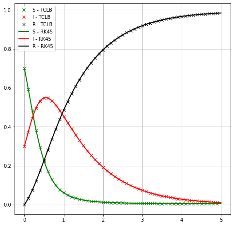
plt.plot(t_lb,S, 'gx', label='S - TCLB')
plt.plot(t_lb,I, 'rx', label='I - TCLB')
plt.plot(t_lb,R, 'kx', label='R - TCLB')

plt.plot(t_rk4, S_rk4,
         color="green", marker="", markevery=1, markersize=15, linestyle="-", linewidth=2,
         label='S - RK45')
plt.plot(t_rk4, I_rk4,
         color="red", marker="", markevery=1, markersize=15, linestyle="-", linewidth=2,
         label='I - RK45')
plt.plot(t_rk4, R_rk4,
         color="black", marker="", markevery=1, markersize=15, linestyle="-", linewidth=2,
         label='R - RK45')
plt.legend()
plt.grid(which='both')

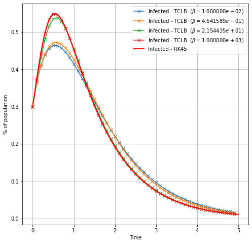
../../_images/15_d2q9_diffusion_SpatialSIR_model_7_0.png

We could use TCLB shortcuts in a loop, to see effects of \(\beta\)¶

plt.figure(figsize=(8,8))
    
for _beta in np.logspace(-5,0,4):
    
    CLBc = CLBXML.CLBConfigWriter( )

    CLBc.addGeomParam('nx', 1)
    CLBc.addGeomParam('ny', 1)


    params = {
            "Diffusivity_W" : 1./6.,
            "Beta_w": (_beta / dt) * dt,
            "Beta":Beta * dt,
            "Gamma":Gamma * dt,            
            "Init_W":I_init, #This is W equation, initlally equall to I. to ensure that large Beta reduces Relaxation-To-SIR Time
            "Init_S":S_init,
            "Init_I":I_init,
            "Init_R":R_init,
            "Init_N":1
    }

    CLBc.addModelParams(params)


    CLBc.addHDF5()
    solve = CLBc.addSolve(iterations=T_lbm)
    CLBc.addHDF5(Iterations=SaveEvery, parent=solve)

    CLBc.write('WSIR-UniformIC-iterBeta.xml')

    ! rm -rf output/* &&  tclb d2q9_reaction_diffusion_system_SIR_ModifiedPeng WSIR-UniformIC-iterBeta.xml > /dev/null && echo "DONE!"


    S = list()
    I = list()
    R = list()
    t_lb = list()
    for i in range(0,T_lbm,SaveEvery):
        f = h5py.File('output/WSIR-UniformIC-iterBeta_HDF5_%08d.h5'%i)    
        #plt.plot(f['DRE_1'][0,25,:])
        S.append( f['S'][0,0,0] )
        I.append( f['I'][0,0,0] )
        R.append( f['R'][0,0,0] )
        t_lb.append(i)

    t_lb = np.array(t_lb)*dt

    plt.plot(t_lb,I, '-x', label=r'Infected - TCLB  ($\beta=%e$)'%(_beta/dt) )

plt.plot(t_rk4, I_rk4,
         color="red", marker="", markevery=1, markersize=15, linestyle="-", linewidth=2,
         label='Infected - RK45')

plt.legend()
plt.grid(which='both')
plt.xlabel('Time')
plt.ylabel('% of population')

Hello allocator!
DONE!
Hello allocator!
DONE!
Hello allocator!
DONE!
Hello allocator!
DONE!

Text(0, 0.5, '% of population')

../../_images/15_d2q9_diffusion_SpatialSIR_model_9_2.png

Modelling of epidemic spreading with Lattice Boltzmann Method

First shot: spatially variable SIR model with uniform IC

Contents

First shot: spatially variable SIR model with uniform IC¶

We could use TCLB shortcuts in a loop, to see effects of \(\beta\)¶

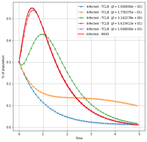
Transition from WSIR to SIR¶

SIR - Simple Laplace¶